Optics in three acts

The following is the script of my latest MSP101 talk. It’s supposed to be an overview of optics covering three different ways to construct them and reason about them. Most of it is devoted to the understanding of Tambara theory and the profunctor encoding, for personal reasons: it’s the last way of thinking about optics that I’ve learned, and it took me the most effort to develop an intuition for them.

In this post I’m assuming basic acquaintance with coend calculus, basically stuff from the first two chapter of ‘Co/end calculus‘. In preparing the talk, I’ve heavily drawn from these papers:

Riley’s ‘Categories of optics‘,
Boisseau’s ‘String diagrams for optics‘,
Gibbons and coauthors’ ‘Profunctor optics: modular data accessors‘,
Pastro & Street’s ‘Doubles for monoidal categories‘,
Roman’s master thesis, which is an amazing compendium of slow-paced theory of optics, ‘Profunctor optics and traversals‘,
and the multiauthor definitive paper on profunctor optics, ‘Profunctor optics: a categorical update‘.

Prelude – Through the looking glass

First of all, what are optics good for? A very partial answer:

Modular data accessors
Optics were born in functional programming from the need of ‘looking inside’ data structures. In particular, they provide a modular abstraction for accessing and updating data structures.
The classic examples are lenses and prisms. Lenses access and update record types, hence components of tuples of types. Prisms access and update ‘corecord’ types, hence coproducts of types.
There are simpler and more complex optics: adapters, simply transform values without dealing with a ‘contextual’ data structure. Traversals access values stored in deeply nested data types like lists, trees, heaps, etc.
Optics were born out of the need of threading together all these kinds of ways to access data, especially for the purpose of being able to composing different flavors of data accessors together. Data is structured in all sorts of bizarre ways (e.g. ‘a tree of pairs of nullables’) and you need to be able to interface different accessors if you want to survive.
An excellent introduction to optics as modular data accessors is the almost-eponymous paper by Gibbons, Pickering and Wu.
Cybernetics
The second area were optics found a home is categorical cybernetics. This because they provide a useful abstraction for bidirectional processes, which cybernetics is full of.
This story basically begins with Jules inventing open games, realising that they amount to indexed families of lenses, and then realising that doesn’t work for Bayesian games: optics were needed in that case, and for completely different reasons than in functional programming. Here, optics are needed to deal with the lack of cartesian structure that lenses need so much. As often happens in category theory, this actually turned out to hint at a much more interesting conceptualization of cybernetic systems and their mathematical models.

Act I – Profunctor representation, or how I stopped worrying and learned to love Tambara modules

Idea

The original (?) definition of optics is through a clever conceptualization of what it means to be an optic, after all. This idea relates to the other two we are going to explore, and it’s surprisingly deep for what has born somewhat as an Haskell hack. In fact, at about the same time profunctor optics were born, Pastro and Street were writing a paper titled ‘Doubles for monoidal categories’ which will turn out ot be extremely relevant. In turn, this paper builds on another work by Tambara published the year before, were he introduces ‘Tambara modules’ as a tool in representation theory. An amazing plot twist!

The crown jewel of Tambara theory (at least as far as opticians are concerned) is the profunctor representation theorem, which provides an explicit characterization of optics, the so-called existential encoding. It can be turned into a slogan as follows: optics are what Tambara modules are presheaves over.

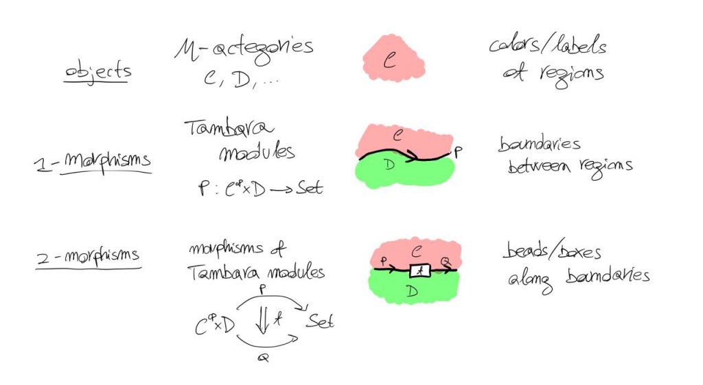
What’s a Tambara module

Tambara modules are ‘just’ strong profunctors, but we need some context to unpack this.
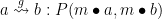
First, let’s fix some data: let $\mathcal C$ , $\mathcal D$ be categories receiving an action of a fixed monoidal category $(\mathcal M, i, \odot)$ . Lately, we’ve been referring to a category equipped with a monoidal action from $\mathcal M$ as ‘actegories’, but in other parts of the literature they’re called ‘ $\mathcal M$ -modules’, generalising the idea that modules in algebra are ‘just’ actions of monoids in the category of abelian groups.

In practice, an action of $\mathcal M$ on $\mathcal C$ allows you to represent objects and morphisms of $\mathcal M$ in $\mathcal C$ (in fact, when some additional structure is around, actions of $\mathcal M$ on $\mathcal C$ are mappings of $\mathcal M$ into $\mathcal C$ ). In symbols, given objects $m:\mathcal M$ and $a:\mathcal C$ , one can write $m \bullet a$ and given $\alpha : m \to n$ , there is a natural transformation $\alpha \bullet - : m \bullet - \to n \bullet -$ . We are going to deal with pairs of actegories over the same monoidal category $\mathcal M$ , and we use the same symbol $\bullet$ to denote all actions.

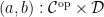
On the other hand, profunctors are the categorification of relations between sets, or more suggestively, they are ‘proof relevant’ relations between categories. A profunctor from 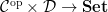$\mathcal C$ to $\mathcal D$ is then a functor $\mathcal C^\mathrm{op} \times \mathcal D \to \mathbf{Set}$ , or a presheaf over $\mathcal C^\mathrm{op} \times \mathcal D$ . Everyone who knows the strict basics of category theory knows at least one profunctor: the Hom profunctor, going from $\mathcal C$ to $\mathcal C$ (in fact, it’s the identity morphisms in the category of categories and profunctors between them).
Indeed, another interpretation of profunctors which is going to play a relevant role here is that they provide a way to talk about morphisms from different categories, aka ‘heteromorphisms’. In fact to give a profunctor $P:\mathcal C \to \mathcal D$ is to answer the question: ‘what’s a morphism from $a:\mathcal C$ to $b:\mathcal D$ like?’ According to $P$ it’s an element $f:P(a,b)$ , which we denote by $f : a \rightsquigarrow b$ . The answer is satisfactory since $P$ has the correct properties you would expect from a hom-like functor, in particular it respects pre-composition with morphisms of $\mathcal C$ and post-composition with morphisms of $\mathcal D$ :

$a' \overset{f}\to a \overset{g}\rightsquigarrow b \overset{h}\to b' : P(a', b')$

Now, Tambara modules are profunctors that, moreover, respect the actegorical structure of $\mathcal C$ and $\mathcal D$ . In fact when that’s present there is one more way to extend a morphism (viz. ‘vertically’):

$m \phantom{\overset{g}\rightsquigarrow} m$
$\bullet \ \phantom{\overset{g}\rightsquigarrow}\ \bullet$
$a \overset{g}\rightsquigarrow b : P(m \bullet a, m \bullet b)$

Functoriality of 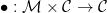$\bullet : \mathcal M \times \mathcal C \to \mathcal C$ makes it obvious that a morphism $f:a \to a'$ of $\mathcal C$ is carried to a new morphism $m \bullet f : m \bullet a \to m \bullet a'$ , but for profunctors, one needs to invoke extra structure. Tambara modules are this, and no more.

Formally, the structure of a Tambara module on $P: \mathcal C \to \mathcal D$ is a family of morphisms (called stregnth)

$\mathrm{st} : P(a,b) \to P(m \bullet a, m \bullet b)$

dinatural in $m$ and natural in $a$ and $b$ , which satisfies reasonable coherence conditions. A morphism of Tambara modules is a natural transformation of presheaves which commutes with the strength.

Each Tambara module is an opinion on the nature of the relation of $\mathcal C$ , $\mathcal D$ and $\mathcal M$ . It proposes ways for a given $a: \mathcal C$ to map into a given $b: \mathcal D$ , and a way for these maps to work with additional context $m:\mathcal M$ around.

Unsurprisingly, the easiest example of Tambara module is the hom-functor of any $\mathcal M$ -actegory. An example of this example is the case where $\mathcal C=\mathcal D=\mathcal M$ is cartesian and acting on itself. In this case, a Tambara module is a so-called cartesian profunctor, then transformations are given by $\mathcal C(a,b)$ and the Tambara structure is given by $\varphi \mapsto 1_m \times \varphi$ .

A less trivial example can be given by non-deterministic maps $\mathcal C(a, Tb)$ where $T$ is a monoidal monad on $\mathcal C$ . Given a context $m:C$ , the Tambara structure now lifts $\varphi : a \to Tb$ to the morphism $m \times a \to T(m \times b)$ obtained by tensoring $\varphi$ with the unit of $T$ and postcomposing with $T$ ‘s monoidal laxator.

Finally, a fortiori, we’ll see ‘universally-many’ Tambara modules can be obtained by considering the representable presheaves on the relevant category of optics as profunctors $\mathcal C \to \mathcal D$ , in particular that of costates when such a thing makes sense.

The Pastro-Street adjunction

As with many structures, one might ask how to I equip the stuff I love with that. In the case of Tambara modules, we ask: if I already have a profunctor $P$ of heteromorphisms I like, can I produce a Tambara module from it in a canonical way? And if yes, how?

The more seasoned category theorists in the audience might already guess there are two answers to this question: one is the ‘minimal’ one and the other is the ‘maximal’ one. Let’s see how they look like.

Since the Tambara structure is a certain compatibility between the action of $m:\mathcal M$ and heteromorphisms $a \rightsquigarrow b$ , one might just think of weeding out all such morphisms that do not respect such a condition when $P$ is equipped with the ‘trivial’ strength, that is, the one that looks for a simple embedding of $P(a,b)$ in $P(m \bullet a,m \bullet b)$ . In other words, we look for the ‘largest subpresheaf’ of $P$ which can be equipped with a strength. A little bit of thinking yields the following definition:

$\Theta P(a,b) = \int_{m: \mathcal M} P(m \bullet a, m \bullet b)$

The only missing idea is realising that $\alpha$ can be given as wedges (see ‘Co/end calculus‘, Definition 1.1.4) for the profunctors $(- \bullet a, - \bullet b) : \mathcal M^\mathrm{op} \times \mathcal M \to \mathbf{Set}$ , naturally indexed by $(a,b):\mathcal C^\mathrm{op} \times \mathcal D$ .

It can be proven quite easily that $\Theta$ is left adjoint to the forgetful functor $U:\mathbf{Tamb}(\mathcal C, \mathcal D) \to \mathbf{Prof}(\mathcal C, \mathcal D)$ , as the category theorists already expected.

But there is also another way to turn a given $P$ into a Tambara module, the ‘maximal’ way. In fact instead of getting rid from $P(a,b)$ of all those heteromorphisms which don’t appear in $P(m \bullet a,m \bullet b)$ , we could forcibly add them to the latter. In other words, we look for the smallest Tambara module containing $P$ . This leads us to another construction, right adjoint to $U$ :

$\Psi P(a,b) = \int^{m:\mathcal M} \int^{x:\mathcal C,y:\mathcal D} C(a, m \bullet x) \times P(x,y) \times D(m \bullet y, b)$

The string of adjoints $\Psi \dashv U \dashv \Theta$ generates an adjoint pair of a comonad $U\Theta$ and a monad $U\Psi$ on $\mathbf{Prof}(\mathcal C,\mathcal D)$ , whose coalgebras and algebras, respectively, coincide and are exactly given by Tambara modules.

(Observation: as we’ll see later, Tambara modules are copresheaves over optics. This gives another characterization/construction for $\Psi$ and $\Theta$ , namely as those functors $\mathbf{Psh}(\mathcal C \times \mathcal D^\mathrm{op}) \to \mathbf{Psh}({\mathcal O_{\bullet, \bullet}}^\mathrm{op})$ induced by the ‘trivial embedding’ functor $\mathcal C \times \mathcal D^\mathrm{op} \to {\mathcal O_{\bullet, \bullet}}^\mathrm{op}$ , i.e. the one sending a pair of morphisms to a residual-less optic).

Profunctor encoding & its explicit representation

We are now ready to define profunctor optics [1]:

$\mathcal O_{\bullet, \bullet}((s,t),(a,b)) := \int_{P : \mathbf{Tamb}(\mathcal C,\mathcal D)} \mathbf{Set}(P(a,b),\,P(s,t))$

If Tambara modules give ‘morphisms’ from $\mathcal C$ to $\mathcal D$ which respect the given action, optics are defined as those transformations which ‘pullback’ these morphisms nicely.

The profunctor encoding selects the minimal common denominator of the opinions each Tambara module express about maps $\mathcal C$ into $\mathcal D$ in order to talk about the morphisms that supposedly respect it.

A neat side-effect of this definition is that profunctor optics can be composed ‘simply by functional composition’, under the end. This is one of the main practical advantages of the profunctor encoding. On the other hand, this definition is problematic because of the non-explicit nature of the encoding. Optics are ‘carved out’ from a very big set, and it’s not clear what the result looks like.

This is when the profunctor representation theorem enters the scene:
$\int_{P : \mathbf{Tamb}(\mathcal C, \mathcal D)} \mathbf{Set}(P(a,b),\,P(s,t)) \cong \int^{m:\mathcal M} \mathcal C(s,m \bullet a) \times \mathcal D(m \bullet b, t)$

The proof consists entirely of applications of the Yoneda lemma:
$\int_{P : \mathbf{Tamb}(\mathcal C,\mathcal D)} \mathbf{Set}(P(a,b),\,P(s,t))$
$= \int_{P : \mathbf{Tamb}(\mathcal C,\mathcal D)} \mathbf{Set}(\mathbf{Prof}(C,D)(y^{(a,b)}, P),\,P(s,t))$
$= \int_{P : \mathbf{Tamb}(\mathcal C,\mathcal D)} \mathbf{Set}(\mathbf{Tamb}(\mathcal C,\mathcal D)(\Psi y^{(a,b)}, P),\,P(s,t))$
$= \Psi y^{(a,b)}(s,t)$
$= \int^{m:\mathcal M} \int^{x:\mathcal C, y:\mathcal D} \mathcal C(s, m \bullet x) \times y^{(a,b)}(x,y) \times \mathcal D(m \bullet y, t)$
$= \int^{m:\mathcal M} \mathcal C(s, m \bullet a) \times \mathcal D(m \bullet b, t)$

A corollary of this theorem is that

$\mathbf{Tamb}(\mathcal C, \mathcal D) \simeq \mathbf{Psh}({\mathcal O_{\bullet,\bullet}}^\mathrm{op})$

In fact:
$\int_{F : \mathbf{Psh}({\mathcal O_{\bullet,\bullet}}^\mathrm{op})} \mathbf{Set}(F(a,b),F(s,t))$
$= \int_{F : \mathbf{Psh}({\mathcal O_{\bullet,\bullet}}^\mathrm{op})} \mathbf{Set}(\mathbf{Psh}({\mathcal O_{\bullet,\bullet}}^\mathrm{op})(y^{(a,b)}, F),\,F(s,t))$
$= y^{(a,b)}(s,t)$
$= \mathcal O_{\bullet,\bullet}((a,b)(s,t))$

The interesting thing is that we can talk about such morphisms despite the fact this mythical Tambara module (the initial Tambara module in the twisted arrow category) does not exist in general.

Coda: hybrid composition

Just a quick observation: the profunctor encoding of optics makes it very explicit that optics of different flavours can be composed in certain cases. In fact, if we have actions $\bullet_{\mathcal M}$ and $\bullet_{\mathcal N}$ of both $\mathcal M$ and $\mathcal N$ on $\mathcal C$ and $\mathcal D$ , then we can produce an action of $\mathcal M + \mathcal N$ on both.

The latter category is made of formal words made by interleaving objects (and morphisms) of the two summands. Analogously, one can use the two original actions to create a ‘coproduct’ action.

Now, evidently, Tambara modules for this action are also Tambara modules for the two original actions, since this action extends both. It turns out that

$\mathbf{Tamb}{(\bullet_{\mathcal M+\mathcal N}, \mathcal C),(\mathcal D, \bullet_{\mathcal M+\mathcal N})} = \mathbf{Tamb}{(\bullet_{\mathcal N}, \mathcal C),(\mathcal D, \bullet_{\mathcal N})} \times_{\mathbf{Prof}} \mathbf{Tamb}{(\bullet_{\mathcal M}, \mathcal C),(\mathcal D, \bullet_{\mathcal M})}$

Therefore profunctor optics for $\bullet_{\mathcal M + \mathcal N} = \bullet_{\mathcal M} + \bullet_{\mathcal N}$ are less ‘picky’ than those for $\mathcal M$ and those for $\mathcal N$ , meaning that taking the end over Tambara modules for the first yields a bigger set than the ones for the latter. All in all, we get embeddings $\mathcal O_{\bullet_{\mathcal M}, \bullet_{\mathcal M}} \longrightarrow \mathcal O_{\bullet_{\mathcal M +\mathcal N}, \bullet_{\mathcal M+\mathcal N}}$
In other words, hybrid composition of optics happens by transporting both flavor of optics to a netural common ground and composing there.

Notice the idea we sketched here is quite more general: if we have a monoidal functor $\phi : \mathcal M \to \mathcal N$ commuting with given actions on $\mathcal C$ and $\mathcal D$ , then we get a morphism $\phi^\bullet : \mathcal O_{\bullet_{\mathcal M}, \bullet_{\mathcal M}} \longrightarrow \mathcal O_{\bullet_{\mathcal N}, \bullet_{\mathcal N}}$ .

The second important side-effect of profunctor encoding is making this composition trivial enough to be inferred by the Haskell compiler (as far as I understand), by exploiting polymorphism. That said, as you see from the above discussion hybrid composition is not an explicit feature of this encoding but can we defined for different encodings as well, albeit less ‘invisibly’.

Act II – Existential optics, or the case for open diagrams

After proving the profunctor representation theorem, one is left with a new, explicit, description of optics

$\mathcal O_{\bullet , \bullet}((s,t),(a,b)) = \int^{m:\mathcal M} C(s,m \bullet a) \times D(m \bullet b, t)$

How to make sense of this? First, let’s look at what this definition actually says: it tells us an optic is given by

a choice of residual $m:\mathcal M$ ,
a map $v: s \to m \bullet a$ in $\mathcal C$ ,
a map $u: m \bullet b \to t$ in $\mathcal D$ ;

quotiented by the equivalence relation induced by the coend, which says morphism $\alpha : m \to m'$ can slide between $v$ and $u$ without changing the optic.

I could write down what this equivalence relation is defined to be in symbols, but it’s much much better to just draw it out. From now on, let’s make a simplification and suppose $\mathcal C = \mathcal D = \mathcal M$ and $\bullet = \odot$ .

In this situation, we can draw all the pieces of an optic as a string diagram in $\mathcal C$ :

It’s almost instictive to join the two wires labelled by $m$ , isn’t it? So, is this instinct backed up by the maths? Yes! Indeed, this is exactly what the sliding relation is telling us to do, albeit enigmatically: it’s telling us that ‘beads’ on the $m$ wire can move freely from one side to the other of the diagram. Topologically, this is allowed iff the wires are connected. Moreover, this move embeds the equivalence relation in the notation itself, a major win.

So we remain with the following picture:

This is called a comb, and as you can see is a kind of wrapper around a morphism $a \to b$ . Indeed, one can still see the shadow of profunctor encoding: an optic is something that ‘wraps’ a transformation $a \rightsquigarrow b$ to yield one $s \rightsquigarrow t$ .
Composition of optics justifies this even further, as this time it’s obtained by nesting combs, as suggested by the wrapping/pull back interpretation.

It’s interesting to notice that, in principle, we are not limited to combs with two teeths only, that is, we could have combs wrapping more than one morphism, which represent computations that yield to the environment at some points, asking it to provide bits of it. Then interleaving combs, so that the teeth of one fill the holes of the another, provides a model of interacting computations (and more than two combs can be involved).

Interleaving is really the most general composition for combs, if we allow for ‘incomplete’ interleaving and ‘degenerate’ ones, that is, if we allow for interleaving to still leave some holes unfilled and if we see connecting combs side to side as a degenerate form of interleaving. This is something Jules (and others, like Davidad as far as I know) has been investigating in the last two years, trying to find a working definition of ‘operad of combs’ with an accompanying coherent diagrammatic language generalising the obvious drawings.

String diagrams for mixed optics

So, we’ve seen optics can be decomposed in three parts: a forward part, a backward part, and a residual wire linking them. The names forward/backward come from the observation that combs look a bit lopsides when it comes to see them as arrows. If we straighten them out:

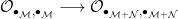
we can see them as morphism in a more conventional way, and we also realize the need to direct the wires of our diagrams: $v$ and $u$ receive data in opposite directions.

This way of drawing optics is key if we want to draw string diagrams for mixed optics, i.e. for those optics where $\mathcal C, \mathcal D$ and $\mathcal M$ do not necessarily coincides.

In fact, as figured out by Guillaume Boisseau, such diagrams can be conveniently interpreted as being drawin in the bicategory of $\mathcal M$ -actegories and Tambara modules between them.

As much as profunctors can be though as ‘generalized functors’ between categories, so can Tambara modules be thought as ‘generalized linear functors’ between actegories (as I said above, both are cases of ‘categoriefied relations’). This means we can compose a Tambara module $\mathcal C \to \mathcal D$ with one $\mathcal D \to \mathcal E$ and obtain one $\mathcal C \to \mathcal E$ . Morphisms between Tambara modules (i.e., natural transformations commuting with the strenghts) make this a bicategory.

This is a good point to remember ourselves that string diagrams are defined for all bicategories, not just monoidal categories (i.e. one-object bicategories). The diagrams are so interpreted:

To draw optics in $\mathbf{Tamb}$ , one embeds $\mathcal C, \mathcal D$ and $\mathcal M$ by using their hom-profunctors. The embeddings for $\mathcal C$ and $\mathcal D$ are given by:
$R_a = \mathcal C(-, {=} \bullet a) : \mathcal C^\mathrm{op} \times \mathcal M \to \mathbf{Set}, \quad L_b = \mathcal D(- \bullet b, =) : \mathcal M^\mathrm{op} \times \mathcal D \to \mathbf{Set}$
whereas $\mathcal M$ is embedded in both ways
$R_m = \mathcal M(-, {=} \bullet m), \quad L_m = \mathcal M(- \bullet m, =)$

Above, $R$ stands for ‘right’ and $L$ stands for ‘left’. This hints at the fact that an object $R_a$ will be drawn as a right-going wire, and an object $L_b$ as a left-going one. You see that we use only one of the two kind of embeddings for $\mathcal C$ and $\mathcal D$ , since their objects have only one direction in $\mathcal O$ , whereas $\mathcal M$ admits both. This fact is very important since $\mathcal M$ becomes the only ‘communication channel’ between the forward and the backward parts. This is corroborated even further by the fact $\mathcal M$ -labelled wires bend:

Counit for $L_m \overset{\mathbf{Tamb}}\dashv R_m$

Counit for $L_m \overset{\mathbf{Tamb}}\dashv R_m$

This bend is actually a (2-)morphism in $\mathbf{Tamb}$ :

$\varepsilon_m : \mathcal M(-, {=} \bullet m) \circ \mathcal M(- \bullet m, =) \to \mathcal M(-, =)$

defined by composition under the coend. Technically speaking, it is the counit of the proadjunction $L_m \overset{\mathbf{Tamb}}\dashv R_m$ (a proadjunction being an adjunction between profunctors):

Now we can finally draw a mixed optic as an honest-to-goodness string diagram in the bicategory of Tambara modules:

Notice that the embeddings we choose, and the shape of the diagrams we draw, are somewhat arbitrary: $\mathcal C$ and $\mathcal D$ also admit embeddings going the opposite way, and $L_x$ is always left adjoint to $R_x$ , no matter where $x$ lives in. So in the bicategory of Tambara modules, we can draw a lot of stuff that ‘violates’ the contract of optics: only $\mathcal M$ can interact with both $\mathcal C$ and $\mathcal D$ at the same time.

This is the essence of the usefulness of optics in cybernetics: they explicitly model bidirectional computation (encoding action-reaction dynamics between a system and its environment) and they do so with an explicit ‘agent subsystem’, whose process theory is given by $\mathcal M$ , expressed by the residual. They are the ones with counits, which are a form of memory. I’ve written more about this here.

Act III – Counits, or how to turn your world upside down

One might take seriously the idea that optics are what you get if you want objects going in two directions and a mediating family of counits which bends the directions. To seriously tackle this intuition, we have again to restrict ourselves to the case $\mathcal C = \mathcal D = \mathcal M$ .

In this case, one can indeed prove that optics is the category obtained by ‘freely addings counits’ to $\mathcal C$ , a fact expressible in the theory of teleological categories. This is our third and final characterization of optics.

Theorem (Riley). Non-mixed optics over a symmetric monoidal category $(\mathcal C, I, \otimes, \sigma)$ are the free teleological category on $\mathcal C$ .
Categories of Optics, Riley

Indeed, a teleological category is a category equipped with a wide subcategory of dualisable objects and morphisms. In non-mixed optics, this is obtained by freely dualising all the morphisms of $\mathcal C$ , which is what happens when we add a ‘backward part’. To account for residuals, we have the second ingredient of a teleological structure: counits, along which dualisable morphisms can slide to become their own duals. In non-mixed optics, residuals have exactly this function, as we notice when we realized optics as open dirgams: they allow sliding from the forward to the backward part.

So one proves Riley’s theorem by ‘surgery’ of a non-mixed optic, realizing it can always be factored in three pieces: a part belonging to $\mathcal C$ , a part belonging to the ‘dual’ and a counit in-between:

Finale

Hopefully, I managed to show you how optics arise in three different ways:

as ‘equivariant transformations’ of data structures,
as open diagrams,
as free categories with counits.

Each of this shows gives optics a certain attitude and adapts to certain intuitions. Observe as only the first two allow to treat the case of mixed optics, while the other way of getting optics is, for now, limited to the ‘non-mixed’ case.

Who knows, perhaps we are going to find a way to extend the last characterization to mixed optics too. It seems possible to define such a thing as a ‘mixed teleological category’, where counits are constructed from actegorical structure. Reasoning about these bends is also central if we want to understand how to syntactically represent iteration (or agent duality) in categories of optics, since unit-like structures seem to be naturally arising from such a proposition.

Footnotes

[1] At MSP we use a different convention on the ‘direction’ of optics, namely that an optic from $(s,t)$ to $(a,b)$ has a forward part going from $s$ to $a$ , instead of the other way around. The latter, adopted in papers such as ‘Profunctor optics: a categorical update‘, is more natural when defining optics via the profunctor encoding, but quite unnatural when using optics as models of interaction.